Towards a Simple Explanation of the Generalization Mystery in Deep Learning
Joint work with Piotr Zielinski
Introduction
Despite the tremendous practical success of deep learning, we do not understand why it works. The problem was highlighted in a beautiful experiment by Zhang et al. in 2016. They took a standard image classification network that performs well on ImageNet, and trained it instead on a modified ImageNet dataset where each image was assigned a random label. By destroying the training signal in this manner, it is clear that there is no hope of correctly labeling test images, but to their surprise – and that of many others – they found that the network still obtains near perfect accuracy in labeling the training images! In other words, the network has sufficient capacity to memorize randomly labeled datasets of ImageNet size.
This simple observation about capacity, they pointed out, posed a challenge to all known explanations of generalization in deep learning and called for a “rethinking” of our approach. After all, if a network has sufficient capacity to memorize random labels, why does it not simply memorize the real ones? This led to a large effort in the machine learning community to better understand why neural networks generalize. Although as a result our understanding has greatly improved, there does not appear to be a satisfactory explanation to date (see Zhang et al. (2021) for a detailed review).
A key problem is that any theory that claims to explain generalization in deep learning cannot be oblivious to the dataset; otherwise it will not be able to explain why there is good generalization on one dataset (real ImageNet) and not in another (random ImageNet). In our recent paper “On the Generalization Mystery in Deep Learning,” we explore a new theory (“Coherent Gradients”) along these lines where the dataset plays a fundamental role in reasoning about generalization.
Gradient Descent and Commonality Exploitation
So why do neural networks generalize on real datasets when they have sufficient capacity to memorize random datasets of the same size? We claim it is because the algorithm used for training – gradient descent (GD) – tries to find and exploit commonality between different training examples during the fitting process. When training examples come from a real dataset (such as ImageNet), they have more in common with each other than when they come from a random dataset (such as the one in Zhang et al.), and we show in our paper that when they have more in common, GD is more stable (in the sense of learning theory) resulting in better generalization (that is, a smaller difference between training and test performance).
But how does GD extract commonality? Recall that GD fits the training set by iteratively taking a small step in a direction that minimizes the average loss across the set (or a sample). This direction is given by the average of the gradients of individual training examples. So, if any commonality is to be extracted between examples, it must be due to averaging since in general there is no other way for examples to interact.
Now, observe that if the gradients of different examples agree in certain components (directions) and disagree in others, then average is stronger in those components than in the others. Thus, the changes to the parameters of the network are biased to preferably fit multiple examples whenever possible. This is illustrated in Figure 1.
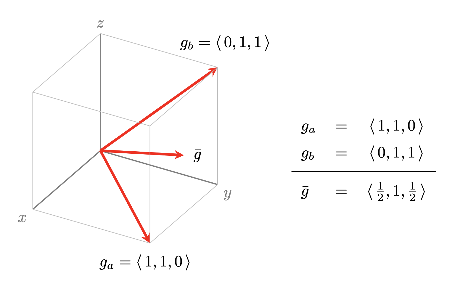
Figure 1. Example showing two training examples $a$ and $b$ whose gradients have a direction in common. Note that the descent step due to the average gradient $\bar{g}$ is stronger in the common direction $y$ (that reduces loss on both $a$ and $b$) than in the idiosyncratic directions $x$ and $z$ (which only reduce loss on one example).
Furthermore, in deep networks, this amplification of gradient components common to multiple examples can become very strong during training due to positive feedback loops between layers, leading to “selection” of features that generalize well. Please see our paper for more details.
Coherence and the difference between Real and Random Data
When gradients of different examples reinforce each other we say they are “coherent,” and use the term “coherence” to informally refer to the alignment or agreement of overall (or components of) per-example gradients. It is possible that there are no components where different per-example gradients add up – this corresponds to fitting each example independently, that is, to “brute force” memorization – and intuitively, we expect this in random datasets (see Figure 2).
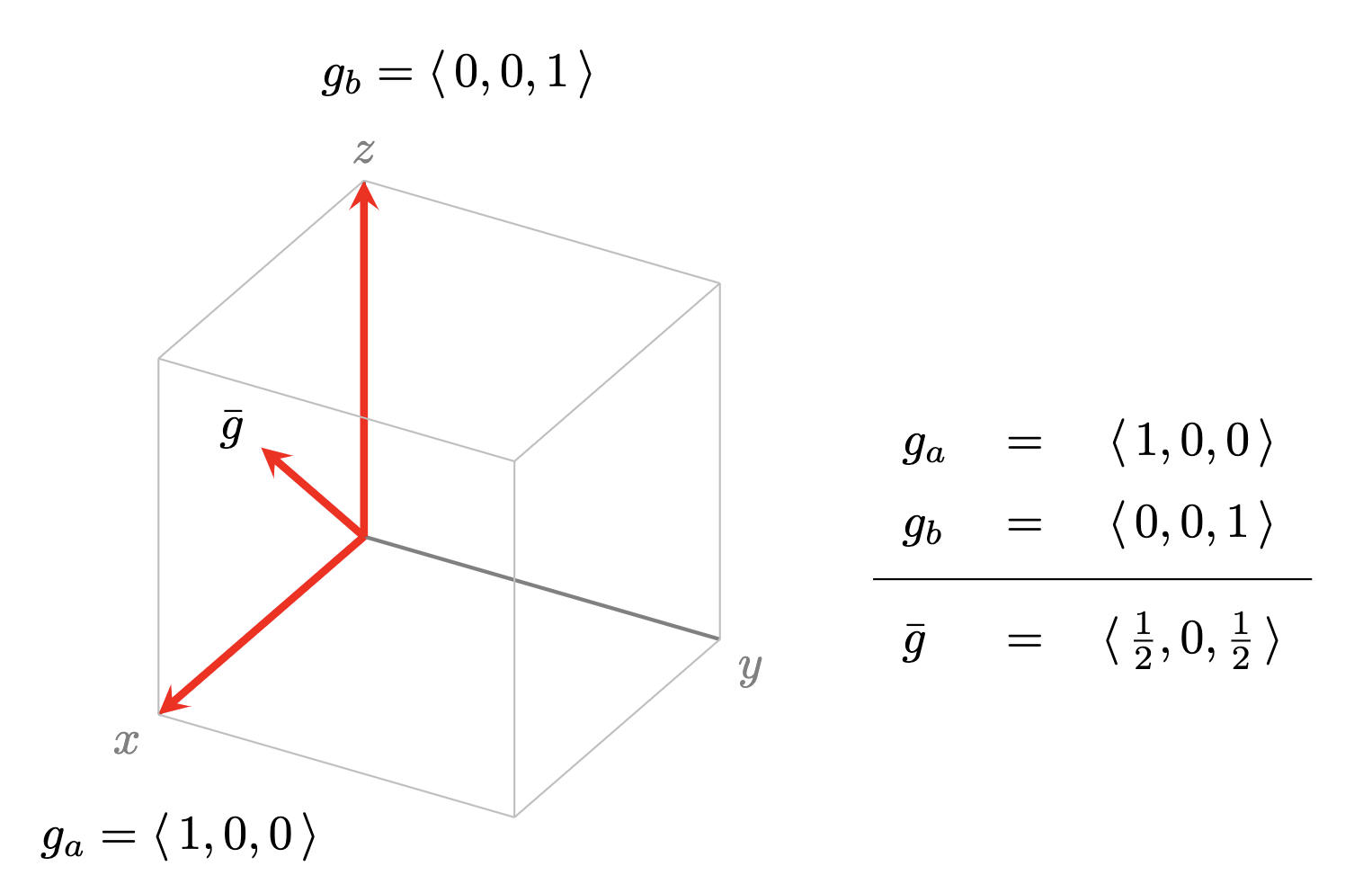
Figure 2. If the gradients of the training examples do not have any common component, that is, they are orthogonal, then the GD step still reduces loss on each example but without extracting commonality (“brute force” memorization).
A natural metric for coherence is the average (or expected) dot product of per-example gradients, but it is hard to interpret since the dot product has no natural scale: is a value of 18.2 good or bad coherence? However, by dividing the average dot product by the average norm of the per-example gradients, we get a metric (denoted by $\alpha$) that is always between 0 and 1 where 1 indicates perfect coherence.
The metric allows us to (qualitatively) bound the generalization gap when GD is run for $T$ time-steps on a sample of size $m$ by extending the iterative framework for analyzing stability introduced by Hardt et al. (2016) to incorporate data dependence (see Theorem 1 of our paper). (For the experts, since our bound is based on stability and not uniform convergence, we avoid the fatal problem pointed out in Nagarajan and Kolter (2019) and get a directionally correct dependence on $m$; and unlike Hardt et al. the bound does not solely depend on limiting the number of times an example is seen during training, and thus applies uniformly to the stochastic and non-stochastic case.)
For practical measurements of coherence, we can further improve interpretability by comparing the coherence of the given sample with that of an hypothetical sample consisting of pairwise orthogonal vectors. Intuitively, this ratio (denoted by $r$) indicates on average how many examples in the sample a given example “helps” during GD. In our experiments, we have found a very significant difference in coherence between real and random datasets across different architectures. An example is shown in Figure 3.
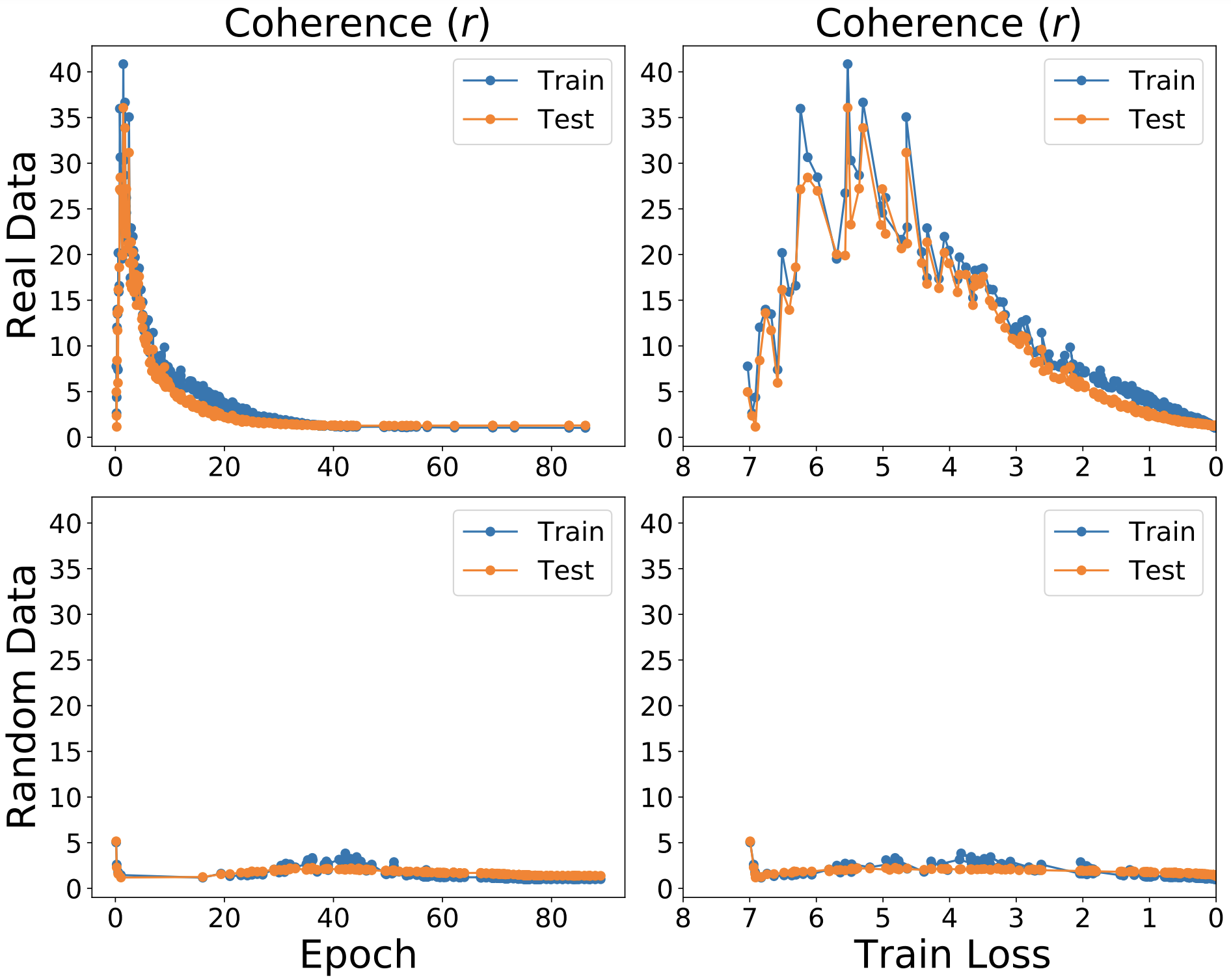
Figure 3. Coherence during training on 50,000 training and test images for a ResNet50 model on real and random ImageNet (top and bottom rows, respectively) as a function of training epoch and training loss (left and right columns). Real ImageNet shows much higher coherence than random with each example helping dozens of other examples in the sample for much of the training. In contrast, each random example helps less than a handful of other examples.
So What?
There are several attractive features of this theory of generalization, some of which we have explored in some detail in our paper, and others whose surface we have barely scratched. First, in addition to the generalization mystery, it explains other intriguing empirical aspects of deep learning such as (1) why some examples are reliably learned earlier than others during training, (2) why learning in the presence of noise labels is possible, (3) why early stopping works, (4) adversarial initialization, and (5) how network depth and width affect generalization.
Second, it is at the right level of generality for a phenomenon as general as generalization in deep learning. It avoids significant pitfalls faced by other theories, and provides an uniform explanation of generalization across various dimensions such as learning and memorization, size and structure of network (from linear regression to deep networks), stochastic and full-batch GD, early stopping and training to convergence, etc.
Finally, since it is a causal (or prescriptive) explanation of generalization, it suggests a simple, yet unexplored, modification to GD to improve generalization: By computing a robust average instead of a simple average of the per-example gradients, the generalization gap (the gap between training and test accuracy) should improve since the weak descent directions are suppressed. A practical experiment based on this idea is shown in Figure 4.
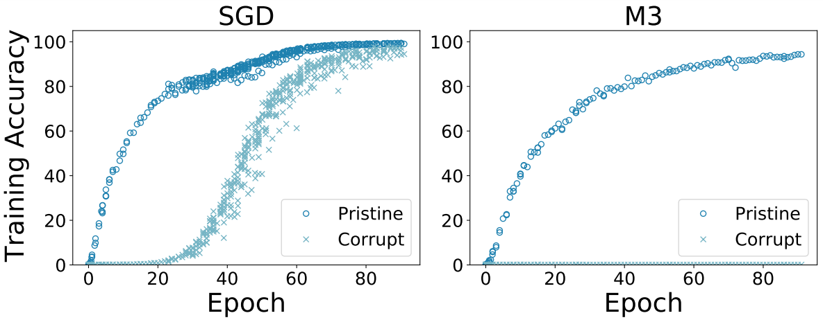
Figure 4. By taking a descent step down the (component-wise) median-of-3 mini-batches (M3) instead of their average as done in Stochastic GD (SGD), the generalization gap can be greatly reduced. For a ResNet50 trained on a dataset where 50% of the images have corrupt labels, SGD learns both pristine and corrupted labels (left) whereas M3 only learns the pristine labels (right).
In conclusion, we hope that our insights into the nature of generalization help practitioners develop a better intuitive understanding of deep learning, and inspire researchers to come up with new algorithms that are more robust, more computationally efficient, and better at preserving privacy than SGD.